📐 信息论与数学工具¶
难度:⭐⭐⭐⭐ | 预计学习时间:6-8小时 | 重要性:理论深度的最后一块拼图
🎯 学习目标¶
- 深入理解互信息、条件熵在特征选择和对比学习中的应用
- 掌握Softmax的温度参数和数值稳定技巧
- 理解反向传播的矩阵推导
- 掌握Attention机制的完整数学推导
1. 信息论进阶¶
1.1 互信息¶
互信息 = 知道Y后,X不确定性减少了多少 = X和Y的依赖程度
import numpy as np
from sklearn.metrics import mutual_info_score
from sklearn.feature_selection import mutual_info_classif

# 互信息用于特征选择(比相关系数更强:能捕捉非线性关系)
np.random.seed(42)
X = np.random.randn(1000, 5)
y = (X[:, 0]**2 + np.sin(X[:, 1]) + 0.1*np.random.randn(1000) > 1).astype(int)

mi_scores = mutual_info_classif(X, y, random_state=42)
for i, score in enumerate(mi_scores):  # enumerate同时获取索引和元素
    print(f"特征{i}: MI={score:.4f} {'← 强相关' if score > 0.1 else ''}")
1.2 条件熵与信息增益¶
信息增益(决策树核心):\(IG(Y, X) = H(Y) - H(Y|X) = I(Y; X)\)
def information_gain(y, x_feature, threshold=None):
    """计算信息增益(决策树分裂准则)"""
    def entropy(labels):
        _, counts = np.unique(labels, return_counts=True)
        probs = counts / len(labels)
        return -np.sum(probs * np.log2(probs + 1e-10))

    parent_entropy = entropy(y)

    if threshold is not None:
        mask = x_feature <= threshold
    else:
        mask = x_feature.astype(bool)

    n = len(y)
    n_left, n_right = mask.sum(), (~mask).sum()

    if n_left == 0 or n_right == 0:
        return 0

    child_entropy = (n_left/n)*entropy(y[mask]) + (n_right/n)*entropy(y[~mask])
    return parent_entropy - child_entropy

# 模拟决策树特征选择
y = np.array([1,1,1,1,0,0,0,0,1,0])
x_good = np.array([1,1,1,1,0,0,0,0,1,0])  # 完美分裂
x_bad  = np.array([1,0,1,0,1,0,1,0,1,0])  # 随机
print(f"好特征信息增益: {information_gain(y, x_good):.4f}")
print(f"差特征信息增益: {information_gain(y, x_bad):.4f}")
1.3 对比学习中的互信息¶
InfoNCE损失与互信息的关系(常见表述):
其中 \(N\) 通常表示正样本与负样本总数(如 \(K+1\))。
import torch
import torch.nn.functional as F

def info_nce_loss(query, positive, negatives, temperature=0.07):
    """InfoNCE损失 — 对比学习核心"""
    # query: [B, D], positive: [B, D], negatives: [B, K, D]
    pos_sim = torch.sum(query * positive, dim=-1) / temperature  # [B]
    neg_sim = torch.bmm(negatives, query.unsqueeze(-1)).squeeze(-1) / temperature  # [B, K]  # unsqueeze增加一个维度  # squeeze去除大小为1的维度

    logits = torch.cat([pos_sim.unsqueeze(-1), neg_sim], dim=-1)  # [B, K+1]
    labels = torch.zeros(query.size(0), dtype=torch.long)  # 正例在第0位

    return F.cross_entropy(logits, labels)

# 实验:温度参数τ对分布的影响
scores = np.array([2.0, 1.5, 0.5, 0.1, -0.5])
for tau in [0.01, 0.07, 0.5, 1.0, 5.0]:
    probs = np.exp(scores / tau) / np.sum(np.exp(scores / tau))
    print(f"τ={tau:.2f}: {np.round(probs, 4)} | 熵={-np.sum(probs*np.log(probs+1e-10)):.4f}")
# τ越小→分布越尖锐(hard),τ越大→分布越平滑(soft)
2. Softmax深入分析¶
2.1 Softmax的温度参数¶
- \(\tau \to 0\):趋近argmax(硬选择)
- \(\tau = 1\):标准softmax
- \(\tau \to \infty\):趋近均匀分布
应用:知识蒸馏中teacher用高温(\(\tau=4\sim20\))产生soft label
2.2 数值稳定的Softmax¶
def stable_softmax(z, temperature=1.0):
    """数值稳定的softmax — 面试必须会"""
    z = np.array(z) / temperature
    z = z - np.max(z)  # 关键:减去最大值防溢出
    exp_z = np.exp(z)
    return exp_z / np.sum(exp_z)

# 不稳定版本会溢出(np.exp(1000)=inf,inf/inf=nan)
z = [1000, 1001, 1002]
naive = np.exp(z) / np.sum(np.exp(z))  # overflow!
print(f"不稳定softmax: {naive}")  # 输出 [nan, nan, nan]

stable = stable_softmax(z)
print(f"稳定softmax: {stable}")  # 正常工作
2.3 Softmax的梯度¶
def softmax_jacobian(z):
    """Softmax的雅可比矩阵"""
    s = stable_softmax(z)
    n = len(s)
    jacobian = np.zeros((n, n))
    for i in range(n):
        for j in range(n):
            if i == j:
                jacobian[i, j] = s[i] * (1 - s[j])
            else:
                jacobian[i, j] = -s[i] * s[j]
    return jacobian

z = [2.0, 1.0, 0.5]
J = softmax_jacobian(z)
print(f"Softmax: {stable_softmax(z)}")
print(f"雅可比矩阵:\n{np.round(J, 4)}")
3. 反向传播的矩阵推导¶

3.1 计算图与链式法则¶
其中 \(\delta^{(l)} = \frac{\partial L}{\partial z^{(l)}}\) 是第\(l\)层的误差信号。
3.2 手写反向传播¶
class ManualMLP:
    """手写两层MLP前向+反向传播"""

    def __init__(self, input_dim, hidden_dim, output_dim):  # __init__构造方法,创建对象时自动调用
        # Xavier初始化
        self.W1 = np.random.randn(input_dim, hidden_dim) * np.sqrt(2.0/(input_dim+hidden_dim))
        self.b1 = np.zeros(hidden_dim)
        self.W2 = np.random.randn(hidden_dim, output_dim) * np.sqrt(2.0/(hidden_dim+output_dim))
        self.b2 = np.zeros(output_dim)

    def relu(self, z):
        return np.maximum(0, z)

    def relu_grad(self, z):
        return (z > 0).astype(float)

    def forward(self, X):
        """前向传播"""
        self.X = X
        self.z1 = X @ self.W1 + self.b1      # [B, H]
        self.a1 = self.relu(self.z1)           # [B, H]
        self.z2 = self.a1 @ self.W2 + self.b2 # [B, O]
        # Softmax
        exp_z = np.exp(self.z2 - np.max(self.z2, axis=1, keepdims=True))
        self.probs = exp_z / np.sum(exp_z, axis=1, keepdims=True)
        return self.probs

    def backward(self, y_onehot, lr=0.01):
        """反向传播 — 面试高频手写题"""
        B = y_onehot.shape[0]

        # 输出层梯度: dL/dz2 = softmax - y (交叉熵+softmax的优美结合)
        delta2 = (self.probs - y_onehot) / B           # [B, O]

        dW2 = self.a1.T @ delta2                        # [H, O]
        db2 = np.sum(delta2, axis=0)                    # [O]

        # 隐藏层梯度
        delta1 = (delta2 @ self.W2.T) * self.relu_grad(self.z1)  # [B, H]

        dW1 = self.X.T @ delta1                         # [D, H]
        db1 = np.sum(delta1, axis=0)                    # [H]

        # 更新
        self.W2 -= lr * dW2
        self.b2 -= lr * db2
        self.W1 -= lr * dW1
        self.b1 -= lr * db1

    def train(self, X, y, epochs=1000, lr=0.01):
        n_classes = len(np.unique(y))
        y_onehot = np.eye(n_classes)[y]

        for epoch in range(epochs):
            probs = self.forward(X)
            loss = -np.mean(np.sum(y_onehot * np.log(probs + 1e-10), axis=1))
            self.backward(y_onehot, lr)  # 反向传播计算梯度

            if epoch % 200 == 0:
                acc = np.mean(np.argmax(probs, axis=1) == y)
                print(f"Epoch {epoch}: loss={loss:.4f}, acc={acc:.4f}")

# 测试
from sklearn.datasets import make_moons
X, y = make_moons(n_samples=300, noise=0.2, random_state=42)
mlp = ManualMLP(2, 32, 2)
mlp.train(X, y, epochs=1000, lr=0.5)
4. Attention机制数学推导¶
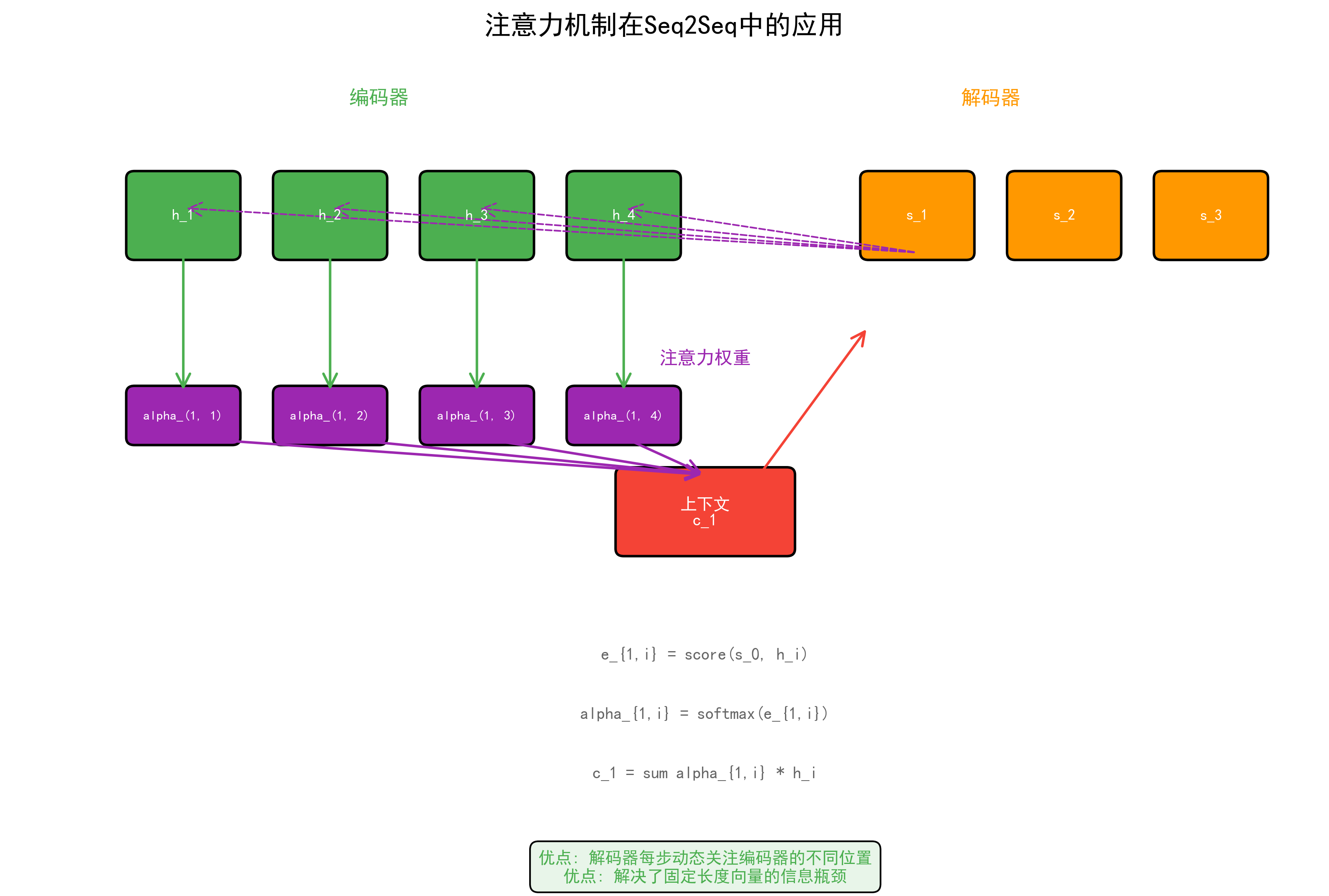
4.1 Scaled Dot-Product Attention¶
为什么除以 \(\sqrt{d_k}\)?
设 \(q, k \in \mathbb{R}^{d_k}\),各分量独立 \(\sim N(0, 1)\),则:
方差随维度线性增长,导致softmax饱和→梯度消失。除以\(\sqrt{d_k}\)使方差归一到1。
import torch
import torch.nn.functional as F

def scaled_dot_product_attention(Q, K, V, mask=None):
    """
    手写Attention — 面试最高频之一
    Q: [B, H, Lq, dk]
    K: [B, H, Lk, dk]
    V: [B, H, Lk, dv]
    """
    dk = Q.size(-1)
    scores = torch.matmul(Q, K.transpose(-2, -1)) / (dk ** 0.5)  # [B,H,Lq,Lk]

    if mask is not None:
        scores = scores.masked_fill(mask == 0, float('-inf'))

    attn_weights = F.softmax(scores, dim=-1)  # [B, H, Lq, Lk]
    output = torch.matmul(attn_weights, V)     # [B, H, Lq, dv]

    return output, attn_weights

# 验证
B, H, L, dk = 2, 4, 8, 64
Q = torch.randn(B, H, L, dk)
K = torch.randn(B, H, L, dk)
V = torch.randn(B, H, L, dk)
out, weights = scaled_dot_product_attention(Q, K, V)
print(f"Output shape: {out.shape}")          # [2, 4, 8, 64]
print(f"Weights sum: {weights.sum(-1)[0,0]}")  # 每行和为1
4.2 Multi-Head Attention¶
class MultiHeadAttention(torch.nn.Module):  # 继承nn.Module定义神经网络层
    """手写Multi-Head Attention"""

    def __init__(self, d_model=512, n_heads=8):
        super().__init__()  # super()调用父类方法
        assert d_model % n_heads == 0  # assert断言,条件为False时抛出异常
        self.d_model = d_model
        self.n_heads = n_heads
        self.dk = d_model // n_heads

        self.W_Q = torch.nn.Linear(d_model, d_model)
        self.W_K = torch.nn.Linear(d_model, d_model)
        self.W_V = torch.nn.Linear(d_model, d_model)
        self.W_O = torch.nn.Linear(d_model, d_model)

    def forward(self, Q, K, V, mask=None):
        B = Q.size(0)

        # 线性投影 + 分头
        Q = self.W_Q(Q).view(B, -1, self.n_heads, self.dk).transpose(1, 2)
        K = self.W_K(K).view(B, -1, self.n_heads, self.dk).transpose(1, 2)
        V = self.W_V(V).view(B, -1, self.n_heads, self.dk).transpose(1, 2)

        # Attention
        out, weights = scaled_dot_product_attention(Q, K, V, mask)

        # 拼接 + 输出投影
        out = out.transpose(1, 2).contiguous().view(B, -1, self.d_model)
        return self.W_O(out)

mha = MultiHeadAttention(d_model=512, n_heads=8)
x = torch.randn(2, 10, 512)
output = mha(x, x, x)
print(f"MHA output: {output.shape}")  # [2, 10, 512]
4.3 位置编码¶

为什么用sin/cos? \(PE_{pos+k}\) 可以表示为 \(PE_{pos}\) 的线性函数,编码了相对位置信息。
import matplotlib.pyplot as plt

def positional_encoding(max_len, d_model):
    """手写位置编码"""
    pe = np.zeros((max_len, d_model))
    position = np.arange(0, max_len)[:, np.newaxis]
    div_term = np.exp(np.arange(0, d_model, 2) * -(np.log(10000.0) / d_model))

    pe[:, 0::2] = np.sin(position * div_term)
    pe[:, 1::2] = np.cos(position * div_term)

    return pe

pe = positional_encoding(100, 512)
plt.figure(figsize=(12, 4))
plt.imshow(pe[:50, :64], aspect='auto', cmap='RdBu')
plt.xlabel("编码维度"); plt.ylabel("位置")
plt.title("位置编码可视化(前50位置, 前64维)")
plt.colorbar(); plt.show()
5. 数学工具速查表¶
5.1 矩阵微积分¶
约定:以下公式采用反向传播(denominator layout)视角,即给出标量损失 \(L\) 对变量的梯度传递规则。前两条本质是链式法则的矩阵形式(已隐含 \(\frac{\partial L}{\partial z}\) 上游梯度),后三条是标准的标量对向量/矩阵求导。
| 表达式 | 梯度/导数 | 备注 |
|---|---|---|
| \(z=Ax\): \(\frac{\partial L}{\partial x}\) | \(A^T \frac{\partial L}{\partial z}\) | 线性层前向,梯度回传 |
| \(z=Ax\): \(\frac{\partial L}{\partial A}\) | \(\frac{\partial L}{\partial z} x^T\) | 权重梯度(外积形式) |
| \(\frac{\partial}{\partial x} x^TAx\) | \((A+A^T)x\) | 二次型(\(A\)对称时为\(2Ax\)) |
| \(\frac{\partial}{\partial X} \text{tr}(AXB)\) | \(A^TB^T\) | 矩阵迹 |
| \(\frac{\partial}{\partial x} \lVert Ax - b\rVert^2\) | \(2A^T(Ax-b)\) | 最小二乘 |
5.2 常用不等式¶
- Jensen不等式:\(f(E[X]) \leq E[f(X)]\)(凸函数),EM算法的理论基础
- Cauchy-Schwarz:\(|E[XY]|^2 \leq E[X^2]E[Y^2]\)
- 信息不等式(KL散度非负性):\(D_{KL}(P\|Q) \geq 0\),等号当且仅当\(P=Q\)
证明思路:\(D_{KL}(P\|Q) = -\sum_x P(x)\log\frac{Q(x)}{P(x)} \geq -\log\sum_x P(x)\cdot\frac{Q(x)}{P(x)} = -\log(1) = 0\)(Jensen不等式,\(\log\) 为凹函数)。详细推导见 02-概率统计 §4.2。
🎓 面试常考题¶
- 为什么Attention要除以√dk? — 防止点积方差随维度增大导致softmax饱和
- 手写反向传播 — 输出层delta=softmax-y,隐藏层delta连乘权重矩阵
- Softmax数值溢出怎么处理? — 减去最大值再exp
- 位置编码为什么用sin/cos? — 线性可表示相对位置,可外推到更长序列
- 互信息和相关系数的区别? — MI能捕捉非线性关系,相关系数只捕捉线性
- 知识蒸馏中温度参数的作用? — 高温使分布平滑,暴露更多类间关系信息
- BatchNorm vs LayerNorm — BN沿batch维归一化(CV),LN沿特征维归一化(NLP/Transformer)
- 为什么交叉熵+softmax求导特别简洁? — \(\frac{\partial L}{\partial z_i} = p_i - y_i\),优美的数学性质
📖 6. 互信息与特征选择¶
6.1 互信息定义¶
互信息衡量两个变量间的非线性依赖关系(比相关系数更通用)。
6.2 基于互信息的特征选择¶
import numpy as np
from sklearn.feature_selection import mutual_info_classif, mutual_info_regression
from sklearn.datasets import make_classification

# 互信息特征选择
X, y = make_classification(n_samples=1000, n_features=20, n_informative=5,
                           n_redundant=5, n_useless=10, random_state=42)

mi_scores = mutual_info_classif(X, y, random_state=42)

# 按互信息排序
feature_ranking = np.argsort(mi_scores)[::-1]
print("特征排名 (按互信息):")
for i, idx in enumerate(feature_ranking[:10]):  # 切片操作取子序列
    print(f"  特征{idx}: MI = {mi_scores[idx]:.4f}")

# 选择MI > 阈值的特征
threshold = 0.05
selected = np.where(mi_scores > threshold)[0]
print(f"\n选择 {len(selected)} / {X.shape[1]} 特征 (阈值={threshold})")
6.3 手写互信息估计(直方图方法)¶
def estimate_mutual_information(x, y, n_bins=30):
    """基于直方图的互信息估计"""
    # 联合分布
    joint_hist, x_edges, y_edges = np.histogram2d(x, y, bins=n_bins)
    joint_prob = joint_hist / joint_hist.sum()

    # 边缘分布
    p_x = joint_prob.sum(axis=1)
    p_y = joint_prob.sum(axis=0)

    # 互信息
    mi = 0.0
    for i in range(n_bins):
        for j in range(n_bins):
            if joint_prob[i, j] > 0 and p_x[i] > 0 and p_y[j] > 0:
                mi += joint_prob[i, j] * np.log(joint_prob[i, j] / (p_x[i] * p_y[j]))

    return mi

# 验证:线性关系 vs 非线性关系
np.random.seed(42)
x = np.random.randn(5000)
y_linear = 2 * x + np.random.randn(5000) * 0.5
y_nonlinear = np.sin(3 * x) + np.random.randn(5000) * 0.3

print(f"线性关系 MI: {estimate_mutual_information(x, y_linear):.4f}")
print(f"非线性关系 MI: {estimate_mutual_information(x, y_nonlinear):.4f}")
print(f"Pearson相关系数(线性): {np.corrcoef(x, y_linear)[0,1]:.4f}")
print(f"Pearson相关系数(非线性): {np.corrcoef(x, y_nonlinear)[0,1]:.4f}")
# 互信息能捕捉非线性关系,Pearson会miss!
📖 7. 对比学习与InfoNCE¶
7.1 InfoNCE损失推导¶
对比学习的目标:最大化正样本对 \((x, x^+)\) 的互信息下界。
给定anchor \(x\),正样本 \(x^+\),\(K\) 个负样本 \(\{x_k^-\}_{k=1}^K\):
为什么叫InfoNCE? 在常见设定下它给出互信息 \(I(x; x^+)\) 的一个下界:
当 \(K \to \infty\),这个下界趋于紧。
7.2 温度参数τ的影响¶
import torch
import torch.nn.functional as F

def info_nce_loss(query, positive, negatives, temperature=0.07):
    """
    InfoNCE对比损失

    Args:
        query: (B, D) anchor编码
        positive: (B, D) 正样本编码
        negatives: (B, K, D) 负样本编码
        temperature: 温度参数
    """
    B, D = query.shape

    # 正样本相似度 (B, 1)
    pos_sim = torch.sum(query * positive, dim=-1, keepdim=True) / temperature

    # 负样本相似度 (B, K)
    neg_sim = torch.bmm(negatives, query.unsqueeze(-1)).squeeze(-1) / temperature

    # InfoNCE = -log(exp(pos) / (exp(pos) + sum(exp(neg))))
    logits = torch.cat([pos_sim, neg_sim], dim=-1)  # (B, 1+K)
    labels = torch.zeros(B, dtype=torch.long)  # 正样本在index 0

    loss = F.cross_entropy(logits, labels)
    return loss

# 测试不同温度的影响
query = F.normalize(torch.randn(32, 128), dim=-1)
positive = F.normalize(query + torch.randn_like(query) * 0.1, dim=-1)
negatives = F.normalize(torch.randn(32, 256, 128), dim=-1)

for tau in [0.01, 0.07, 0.5, 1.0]:
    loss = info_nce_loss(query, positive, negatives, temperature=tau)
    print(f"τ={tau:.2f}: loss={loss.item():.4f}")  # .item()将单元素张量转为Python数值

# τ小 → 分布尖锐,专注于困难负样本
# τ大 → 分布平滑,所有负样本权重接近
📖 8. 扩散模型的信息论视角¶
8.1 前向过程的信息损失¶
扩散模型的前向过程 \(q(x_t|x_{t-1}) = \mathcal{N}(\sqrt{1-\beta_t} x_{t-1}, \beta_t I)\)
每一步增加噪声 = 增加条件熵 \(H(X_t|X_{t-1})\) = 损失互信息 \(I(X_0; X_t) \downarrow\)
当 \(t \to T\)(足够多步),\(I(X_0; X_T) \approx 0\),信息完全丢失,\(X_T \approx \mathcal{N}(0, I)\)
8.2 反向过程的信息恢复¶
反向过程 \(p_\theta(x_{t-1}|x_t)\) 需要从纯噪声中逐步恢复信息:
训练目标(简化版)等价于最小化每一步的"信息恢复错误":
8.3 Score与KL散度的关系¶
Score function \(s_\theta(x, t) = \nabla_x \log p_t(x)\) 的训练可以理解为:
每一步最小化真实条件分布与模型预测分布的KL散度。
import torch

def diffusion_info_analysis(T=1000, beta_start=1e-4, beta_end=0.02):
    """分析扩散过程中的信息损失"""
    betas = torch.linspace(beta_start, beta_end, T)
    alphas = 1 - betas
    alpha_bar = torch.cumprod(alphas, dim=0)

    # 信号与噪声比 (SNR)
    snr = alpha_bar / (1 - alpha_bar)

    # 互信息上界(高斯信道容量)
    mi_upper = 0.5 * torch.log(1 + snr)

    print(f"t=0:   SNR={snr[0]:.2f},   MI上界={mi_upper[0]:.4f} nats")
    print(f"t=250: SNR={snr[250]:.4f}, MI上界={mi_upper[250]:.4f} nats")
    print(f"t=500: SNR={snr[500]:.6f}, MI上界={mi_upper[500]:.4f} nats")
    print(f"t=999: SNR={snr[999]:.8f}, MI上界={mi_upper[999]:.6f} nats")

    # 信息损失最快的区间
    mi_diff = -torch.diff(mi_upper)
    peak_loss_t = mi_diff.argmax().item()
    print(f"\n信息损失最快的时间步: t={peak_loss_t}")
    print(f"这对应DDPM在此时间步附近采样最关键")

diffusion_info_analysis()
🎯 面试高频题(扩展)¶
- 互信息和相关系数的区别? — 相关系数只捕捉线性关系,互信息捕捉任意非线性依赖。MI=0⇔独立,相关=0只说明无线性关系
- InfoNCE为什么需要大batch的负样本? — 负样本越多,MI下界越紧;实践中常用较大的batch来提升效果,因为\(\log(K)\)增长缓慢
- 对比学习中温度τ怎么选? — τ小(0.01-0.1)关注困难负样本(hard negatives),易过拟合;τ大(0.5-1.0)学更均匀表示。一般0.07-0.1
- 扩散模型的损失函数本质是什么? — 每一步的去噪预测误差,等价于最小化变分下界(VLB)中各时间步的KL散度之和
- 什么是Score Matching? — 学习数据分布的梯度\(\nabla_x \log p(x)\)(score),不需知道归一化常数。扩散模型、能量模型的训练基础
- 特征选择为什么不能只看单特征MI? — 单特征MI忽略特征间冗余。特征A和B各自MI都高,但信息重叠。需要用条件MI或mRMR方法
✅ 学习检查清单¶
- 能计算互信息并解释其在特征选择中的应用
- 能写出数值稳定的softmax实现
- 能手推两层MLP的反向传播(矩阵形式)
- 能完整写出Scaled Dot-Product Attention
- 能解释 \(\sqrt{d_k}\) 缩放的原因
- 能实现Multi-Head Attention
- 能写出位置编码公式并解释原理