01-循环神经网络基础
学习时间: 约6-8小时 难度级别: ⭐⭐⭐⭐ 中高级 前置知识: 神经网络基础、反向传播算法、PyTorch基础 学习目标: 理解RNN/LSTM/GRU的原理与数学推导,掌握PyTorch实现
目录
- 1. 序列数据与循环网络动机
- 2. 基础RNN原理
- 3. BPTT算法
- 4. 梯度消失与梯度爆炸
- 5. LSTM详解
- 6. GRU详解
- 7. 双向RNN与多层RNN
- 8. PyTorch完整实现
- 9. 练习与自我检查
1. 序列数据与循环网络动机
1.1 序列数据的特点
- 可变长度: 不同句子长度不同
- 顺序依赖: "我爱你" ≠ "你爱我"
- 长距离依赖: 句首的词可能影响句末的意思
1.2 为什么全连接网络不适合
- 无法处理可变长度输入
- 不共享跨时间步的参数
- 参数量随序列长度爆炸增长
2. 基础RNN原理
2.1 RNN展开图
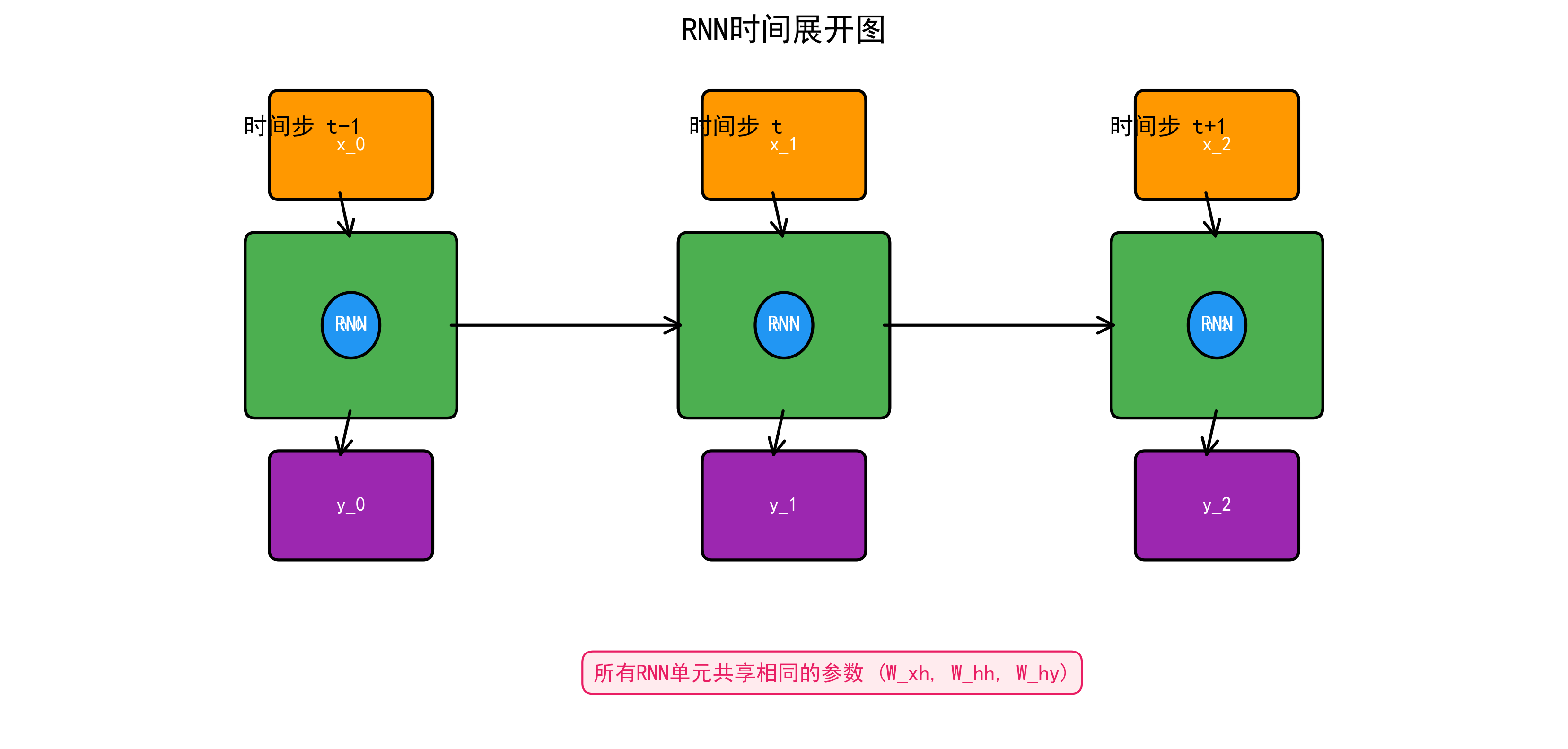
RNN在时间轴上展开后的结构如图所示,每个时间步共享相同的参数。
其中: - \(x_t \in \mathbb{R}^d\): 时间步 \(t\) 的输入 - \(h_t \in \mathbb{R}^h\): 时间步 \(t\) 的隐藏状态 - \(W_{xh} \in \mathbb{R}^{h \times d}\): 输入到隐藏的权重 - \(W_{hh} \in \mathbb{R}^{h \times h}\): 隐藏到隐藏的权重 - \(W_{hy} \in \mathbb{R}^{o \times h}\): 隐藏到输出的权重
关键特性:所有时间步共享同一组参数 \(W_{xh}, W_{hh}, W_{hy}\)。
2.2 手动实现RNN
import torch
import torch.nn as nn

class ManualRNNCell(nn.Module):  # 继承nn.Module定义神经网络层
    """手动实现 RNN Cell"""
    def __init__(self, input_size, hidden_size):  # __init__构造方法,创建对象时自动调用
        super().__init__()  # super()调用父类方法
        self.hidden_size = hidden_size

        # 参数
        self.W_xh = nn.Parameter(torch.randn(input_size, hidden_size) * 0.01)
        self.W_hh = nn.Parameter(torch.randn(hidden_size, hidden_size) * 0.01)
        self.b_h = nn.Parameter(torch.zeros(hidden_size))

    def forward(self, x_t, h_prev):
        """
        x_t: (batch, input_size) 当前时间步输入
        h_prev: (batch, hidden_size) 上一个隐藏状态
        """
        h_t = torch.tanh(x_t @ self.W_xh + h_prev @ self.W_hh + self.b_h)
        return h_t

class ManualRNN(nn.Module):
    """手动实现完整 RNN"""
    def __init__(self, input_size, hidden_size, num_classes):
        super().__init__()
        self.hidden_size = hidden_size
        self.rnn_cell = ManualRNNCell(input_size, hidden_size)
        self.fc = nn.Linear(hidden_size, num_classes)

    def forward(self, x, h_0=None):
        """
        x: (batch, seq_len, input_size)
        """
        batch_size, seq_len, _ = x.shape

        if h_0 is None:
            h_0 = torch.zeros(batch_size, self.hidden_size, device=x.device)

        h_t = h_0
        outputs = []
        for t in range(seq_len):
            h_t = self.rnn_cell(x[:, t, :], h_t)
            outputs.append(h_t)

        # outputs: list of (batch, hidden_size)
        outputs = torch.stack(outputs, dim=1)  # (batch, seq_len, hidden_size)

        # 取最后一个时间步的输出进行分类
        out = self.fc(h_t)
        return out, outputs

# 测试
model = ManualRNN(input_size=10, hidden_size=64, num_classes=5)
x = torch.randn(32, 20, 10)  # batch=32, seq_len=20, input=10
out, all_hidden = model(x)
print(f"输出: {out.shape}, 所有隐藏状态: {all_hidden.shape}")
3. BPTT算法
3.1 时间反向传播(Backpropagation Through Time)
RNN的训练使用BPTT算法 — 将RNN在时间轴上展开后应用标准反向传播。
总损失为各时间步损失之和: $\(\mathcal{L} = \sum_{t=1}^{T} \mathcal{L}_t\)$
对 \(W_{hh}\) 的梯度涉及对所有时间步的求和:
3.2 截断BPTT
为了控制计算成本和数值稳定性,实践中通常使用截断BPTT — 只在固定长度的片段内做反向传播。
def truncated_bptt_training(model, data_stream, seq_length=35, optimizer=None, criterion=None):
    """截断 BPTT 训练"""
    h = None
    for i in range(0, len(data_stream) - 1, seq_length):
        # 获取片段
        x = data_stream[i:i+seq_length]
        y = data_stream[i+1:i+seq_length+1]

        # 截断梯度链,但保留隐藏状态值
        if h is not None:
            h = h.detach()  # detach()从计算图分离,不参与梯度计算

        output, h = model(x, h)
        loss = criterion(output.view(-1, output.size(-1)), y.view(-1))  # view重塑张量形状(要求内存连续)

        optimizer.zero_grad()  # 清零梯度,防止梯度累积
        loss.backward()  # 反向传播计算梯度
        torch.nn.utils.clip_grad_norm_(model.parameters(), max_norm=5.0)
        optimizer.step()  # 根据梯度更新模型参数
4. 梯度消失与梯度爆炸

4.1 问题分析
从 BPTT 的梯度公式中,关键项是:
设 \(W_{hh}\) 的最大特征值为 \(\lambda_{\max}\):
- 若 \(\lambda_{\max} \cdot \max(1 - h_j^2) < 1\),连乘趋向 0 → 梯度消失
- 若 \(\lambda_{\max} \cdot \max(1 - h_j^2) > 1\),连乘趋向 ∞ → 梯度爆炸
4.2 后果
- 梯度消失: 模型无法学习长距离依赖关系
- 梯度爆炸: 参数更新过大,训练发散
4.3 解决方案
| 问题 | 解决方案 |
|---|---|
| 梯度爆炸 | 梯度裁剪 |
| 梯度消失 | LSTM/GRU(门控机制) |
| 梯度消失 | 残差连接 |
| 梯度消失 | 使用ReLU代替Tanh |
5. LSTM详解

5.1 核心思想
Long Short-Term Memory(Hochreiter & Schmidhuber, 1997)通过门控机制和细胞状态解决长距离依赖问题。
核心创新:引入细胞状态 \(C_t\)作为信息的"传送带",通过三个门控制信息的流入、流出和遗忘。
5.2 门控机制数学推导
遗忘门(Forget Gate):决定保留多少旧的细胞状态 $\(f_t = \sigma(W_f [h_{t-1}, x_t] + b_f)\)$
输入门(Input Gate):决定添加多少新信息 $\(i_t = \sigma(W_i [h_{t-1}, x_t] + b_i)\)$
候选细胞状态:生成新的候选信息 $\(\tilde{C}_t = \tanh(W_C [h_{t-1}, x_t] + b_C)\)$
细胞状态更新: $\(C_t = f_t \odot C_{t-1} + i_t \odot \tilde{C}_t\)$
输出门(Output Gate):决定输出多少当前细胞状态 $\(o_t = \sigma(W_o [h_{t-1}, x_t] + b_o)\)$
隐藏状态: $\(h_t = o_t \odot \tanh(C_t)\)$
5.3 为什么LSTM能缓解梯度消失
细胞状态的梯度传播:
当 \(f_t \approx 1\)(遗忘门接近1),梯度可以"无损"地传递回去。这就像一条"梯度高速公路"。
5.4 PyTorch实现
class ManualLSTMCell(nn.Module):
    """手动实现 LSTM Cell"""
    def __init__(self, input_size, hidden_size):
        super().__init__()
        self.hidden_size = hidden_size

        # 将四个门的参数合并为一个大矩阵以提高效率
        self.linear_ih = nn.Linear(input_size, 4 * hidden_size)
        self.linear_hh = nn.Linear(hidden_size, 4 * hidden_size)

    def forward(self, x_t, state):
        """
        x_t: (batch, input_size)
        state: (h_prev, c_prev) 各 (batch, hidden_size)
        """
        h_prev, c_prev = state

        # 一次计算四个门
        gates = self.linear_ih(x_t) + self.linear_hh(h_prev)

        # 分割
        i_gate, f_gate, g_gate, o_gate = gates.chunk(4, dim=1)

        # 激活
        i_t = torch.sigmoid(i_gate)      # 输入门
        f_t = torch.sigmoid(f_gate)      # 遗忘门
        g_t = torch.tanh(g_gate)         # 候选细胞
        o_t = torch.sigmoid(o_gate)      # 输出门

        # 更新细胞状态
        c_t = f_t * c_prev + i_t * g_t

        # 计算隐藏状态
        h_t = o_t * torch.tanh(c_t)

        return h_t, c_t

class ManualLSTM(nn.Module):
    """手动实现完整 LSTM"""
    def __init__(self, input_size, hidden_size, num_layers=1):
        super().__init__()
        self.hidden_size = hidden_size
        self.num_layers = num_layers

        self.cells = nn.ModuleList([
            ManualLSTMCell(
                input_size if i == 0 else hidden_size,
                hidden_size
            )
            for i in range(num_layers)
        ])

    def forward(self, x, initial_state=None):
        """
        x: (batch, seq_len, input_size)
        """
        batch_size, seq_len, _ = x.shape

        if initial_state is None:
            h = [torch.zeros(batch_size, self.hidden_size, device=x.device) for _ in range(self.num_layers)]  # 列表推导式,简洁创建列表
            c = [torch.zeros(batch_size, self.hidden_size, device=x.device) for _ in range(self.num_layers)]
        else:
            h, c = initial_state
            h = [h[i] for i in range(self.num_layers)]
            c = [c[i] for i in range(self.num_layers)]

        outputs = []
        for t in range(seq_len):
            layer_input = x[:, t, :]
            for layer_idx, cell in enumerate(self.cells):  # enumerate同时获取索引和元素
                h[layer_idx], c[layer_idx] = cell(layer_input, (h[layer_idx], c[layer_idx]))
                layer_input = h[layer_idx]
            outputs.append(h[-1])  # [-1]负索引取最后一个元素

        outputs = torch.stack(outputs, dim=1)
        return outputs, (torch.stack(h), torch.stack(c))

# 使用 PyTorch 内置 LSTM
lstm = nn.LSTM(
    input_size=100,    # 输入特征维度
    hidden_size=256,   # 隐藏状态维度
    num_layers=2,      # 层数
    batch_first=True,  # 输入 shape: (batch, seq, feature)
    dropout=0.5,       # 层间 dropout
    bidirectional=False
)

x = torch.randn(32, 50, 100)
output, (h_n, c_n) = lstm(x)
print(f"输出: {output.shape}")  # (32, 50, 256)
print(f"最终隐藏: {h_n.shape}") # (2, 32, 256) — num_layers × batch × hidden
print(f"最终细胞: {c_n.shape}") # (2, 32, 256)
6. GRU详解

6.1 GRU原理
Gated Recurrent Unit(Cho et al., 2014)简化了 LSTM,将遗忘门和输入门合并为更新门,取消了独立的细胞状态。
重置门(Reset Gate): $\(r_t = \sigma(W_r [h_{t-1}, x_t] + b_r)\)$
更新门(Update Gate): $\(z_t = \sigma(W_z [h_{t-1}, x_t] + b_z)\)$
候选隐藏状态: $\(\tilde{h}_t = \tanh(W_h [r_t \odot h_{t-1}, x_t] + b_h)\)$
隐藏状态更新: $\(h_t = (1 - z_t) \odot h_{t-1} + z_t \odot \tilde{h}_t\)$
6.2 GRU vs LSTM
| 特性 | LSTM | GRU |
|---|---|---|
| 门的数量 | 3 (遗忘/输入/输出) | 2 (重置/更新) |
| 参数量 | \(4h(h+d)\) | \(3h(h+d)\) |
| 细胞状态 | 独立的 \(C_t\) | 无,只有 \(h_t\) |
| 性能 | 通常更强(长序列) | 短序列表现相当 |
| 训练速度 | 较慢 | 较快 |
# PyTorch GRU
gru = nn.GRU(
    input_size=100,
    hidden_size=256,
    num_layers=2,
    batch_first=True,
    dropout=0.5
)

x = torch.randn(32, 50, 100)
output, h_n = gru(x)
print(f"GRU 输出: {output.shape}")    # (32, 50, 256)
print(f"GRU 隐藏: {h_n.shape}")       # (2, 32, 256)
7. 双向RNN与多层RNN

7.1 双向RNN
同时从前向和后向处理序列,捕获双向上下文:
# 双向 LSTM
bilstm = nn.LSTM(
    input_size=100,
    hidden_size=256,
    num_layers=2,
    batch_first=True,
    bidirectional=True  # 双向
)

x = torch.randn(32, 50, 100)
output, (h_n, c_n) = bilstm(x)
print(f"BiLSTM 输出: {output.shape}")  # (32, 50, 512) — 512 = 256 * 2
print(f"BiLSTM h_n: {h_n.shape}")     # (4, 32, 256) — 4 = 2layers * 2directions
7.2 多层RNN
堆叠多层RNN增加模型容量。下一层的输入是上一层的输出序列。
class StackedLSTM(nn.Module):
    """带层间dropout的多层LSTM"""
    def __init__(self, input_size, hidden_size, num_layers, dropout=0.5):
        super().__init__()
        self.layers = nn.ModuleList()
        self.dropouts = nn.ModuleList()

        for i in range(num_layers):
            self.layers.append(nn.LSTM(
                input_size if i == 0 else hidden_size,
                hidden_size,
                batch_first=True
            ))
            if i < num_layers - 1:
                self.dropouts.append(nn.Dropout(dropout))

    def forward(self, x):
        for i, layer in enumerate(self.layers):
            x, _ = layer(x)
            if i < len(self.dropouts):
                x = self.dropouts[i](x)
        return x
8. PyTorch完整实现
class TextClassifier(nn.Module):
    """基于LSTM的文本分类模型"""
    def __init__(self, vocab_size, embed_dim, hidden_dim, num_classes,
                 num_layers=2, bidirectional=True, dropout=0.5, pad_idx=0):
        super().__init__()
        self.embedding = nn.Embedding(vocab_size, embed_dim, padding_idx=pad_idx)
        self.lstm = nn.LSTM(
            embed_dim, hidden_dim, num_layers,
            batch_first=True, bidirectional=bidirectional, dropout=dropout
        )
        self.dropout = nn.Dropout(dropout)
        direction = 2 if bidirectional else 1
        self.fc = nn.Linear(hidden_dim * direction, num_classes)

    def forward(self, x, lengths=None):
        # x: (batch, seq_len)
        embedded = self.dropout(self.embedding(x))

        if lengths is not None:
            packed = nn.utils.rnn.pack_padded_sequence(
                embedded, lengths.cpu(), batch_first=True, enforce_sorted=False
            )
            output, (h_n, c_n) = self.lstm(packed)
            output, _ = nn.utils.rnn.pad_packed_sequence(output, batch_first=True)
        else:
            output, (h_n, c_n) = self.lstm(embedded)

        # 取最后时间步 (前向最后 + 后向最后)
        if self.lstm.bidirectional:
            hidden = torch.cat([h_n[-2], h_n[-1]], dim=1)
        else:
            hidden = h_n[-1]

        return self.fc(self.dropout(hidden))

# 使用
model = TextClassifier(
    vocab_size=10000, embed_dim=300, hidden_dim=256,
    num_classes=2, num_layers=2, bidirectional=True
)
x = torch.randint(0, 10000, (32, 100))
lengths = torch.randint(10, 100, (32,))
output = model(x, lengths)
print(f"分类输出: {output.shape}")  # (32, 2)
9. 练习与自我检查
练习题
- 手动实现RNN:从零实现简单RNN,在字符级语言模型上训练,生成一小段文本。
- 梯度分析:训练一个深层RNN,监控不同时间步的梯度范数,验证梯度消失问题。
- LSTM vs GRU:在同一任务上对比LSTM和GRU的性能和训练速度。
- 双向LSTM:实现基于BiLSTM的命名实体识别模型。
- 变长序列:使用
pack_padded_sequence正确处理变长序列输入。
自我检查清单
- 能画出RNN的展开图并写出数学公式
- 理解BPTT算法的推导
- 能解释梯度消失/爆炸的根本原因
- 能详细描述LSTM的三个门控机制
- 理解LSTM为什么能缓解梯度消失
- 了解GRU与LSTM的区别和适用场景
- 能实现双向、多层LSTM
- 掌握PyTorch中
pack_padded_sequence的使用
下一篇: 02-序列建模实战 — RNN 在文本分类、序列生成等任务中的实战